Statbotics

The EPA Model

The Expected Points Added (EPA) model builds upon the Elo rating system, but transforms ratings to point units and makes several modifications

Motivation

Prior to 2023, Statbotics displayed both Elo and OPR ratings for each team. OPR was separated into Auto, Teleop, and Endgame components, while sorting was primarily done on Elo, the more predictive model. Match predictions were made by averaging the win probabilities from each model, which slightly outperformed either model individually. The complexity of this setup was not ideal, and resulted in reduced data freshness and inconsistent sorting/component contributions. The EPA model was developed to replace both Elo and OPR with a single unified system. At a high level, the EPA model converts Elo into point contributions, and then makes several modifications to improve accuracy and interpretability. In this article, I'll dive into the details of the EPA model, and how it compares to existing approaches.

Derivation from Elo

As alluded to above, the EPA model builds upon the Elo rating system. But what is Elo, and how exactly does it work, especially for FRC? The Elo rating system is a well-known method for ranking chess players, and has been adapted to many other domains. Each player is given an initial rating, and then the rating is updated after each game depending on the predicted and actual outcome. Several modifications have been made to adapt Elo for use in FRC, specifically to handle alliances, incorporate winning margin, and account for a new game each year.

Recapping Elo

Each team starts with an Elo rating of 1500. An alliance's rating is the sum of the ratings of its three teams. To predict the winner of a match, the Elo ratings of the two alliances are compared. The win probability is a logistic function of the difference between the two ratings:

$P_{win} = \frac{1}{1 + 10^{\frac{d}{400}}}$

where

$d$

is the difference between the two ratings.

After the match, the rating of each team on the winning alliance is increased, and the rating of each team on the losing alliance is decreased. The amount of change is proportional to the surprise of the outcome. Since each year is a new game, scoring must be standardized into consistent units. This is done by dividing by the standard deviation of Week 1 scores. The predicted score margin is defined as 0.004 times the difference in ratings, and the actual score margin is the difference between actual scores divided by the standard deviation. The amount of change is then proportional to the difference between the predicted and actual score margins:

$\text{Predicted Score Margin} = 0.004 \times (\text{Red Rating} - \text{Blue Rating})$

$\text{Actual Score Margin} = \frac{\text{Red Score} - \text{Blue Score}}{\sigma}$

$\Delta R = K \times (\text{Actual Score Margin} - \text{Predicted Score Margin})$

where

$K$

is a constant that controls the amount of change. K is set to 12 for qualification matches and 3 for playoff matches. Small adjustments are made to penalize rookie teams and apply mean reversion year over year. For its relative simplicity, Elo has proven to be a very effective model for FRC.

Point Unit Elo

I set out to convert Elo ratings from arbitrary units into year-specific points. Instead of setting the initial rating to 1500, I set it to one third of the average score in Week 1. The alliance rating is the sum of the team ratings, and doubles as the predicted alliance score. The predicted score margin is then the difference between the two alliance scores, and the actual score margin is the difference between the actual scores. Both require no additional scaling, and are in the same units as the scores. All that is left is to update the ratings after each match.

Suppose two alliances have a rating difference of X, but play a match consistent with a rating difference of Y. The predicted score margin is

$0.004 \times X$

, and the actual score margin is

$0.004 \times Y$

. The surprise of the outcome, measured in standard deviations is

$\frac{(Y - X)}{250}$

. Each team's rating is updated by

$K \times \frac{(Y - X)}{250}$

With three teams on each alliance, the new rating difference is

$X + 6 \times K \times \frac{(Y - X)}{250}$

. The difference between the new and old rating difference is

$6 \times K \times \frac{(Y - X)}{250}$

. Substituting

$K=12$

, Elo updates ratings by

$\frac{72}{250}\approx29\%$

of the difference between the current and observed ratings.

Extending this approach to the EPA model, each team's EPA is updated according to the equations below:

$\text{Predicted Score Margin} = \text{Red EPA} - \text{Blue EPA}$

$\text{Actual Score Margin} = \text{Red Score} - \text{Blue Score}$

$\Delta EPA = \frac{72}{250} \times (\text{Actual Score Margin} - \text{Predicted Score Margin})$

So far, the EPA model is identical to the Elo model, with the only modification being a unit conversion. Interestingly, this new update step is just an exponential moving average.

Modifications

No longer zero-sum

First, a conceptual point. Elo is inherently zero-sum, meaning that the sum of the ratings of all teams is constant. For a team's rating to increase, another team's rating must decrease. As the season progresses, the average match score increases, but the average rating does not (ignoring selection bias in district championships onwards). This means an Elo of 1500 in Week 1 is not the same as an Elo of 1500 in Week 5. The EPA model is conciously designed to not be zero-sum, so that the average rating is meaningful and increases as the season progresses. Instead of computing the rating update, and spreading it across the alliance, the EPA update is computed for each team individually. This allows modifications to the update function on a per-team basis.

Updating the K parameter

The K paramater (originally

$\frac{72}{250}$

) is very well tuned, but a little slow to adjust early in the season. I instead use a piecewise linear function of the number of matches played to scale the update factor

$K$

$K = \begin{cases} 0.5 & N \leq 6 \\ 0.5 - \frac{1}{30}\times(N-6) & 6 < N \leq 12 \\ 0.3 & N > 12 \end{cases}$

Introducing the Margin parameter

Substituting in the expressions for predicted score margin and actual score margin,

$\Delta EPA = K \times (\text{Red Score} - \text{Blue Score} - (\text{Red EPA} - \text{Blue EPA}))$

$\Delta EPA = K \times ((\text{Red Score} - \text{Red EPA}) - (\text{Blue Score} - \text{Blue EPA}))$

Where

$N$

is the number of qualification matches played.

The initial explanation of the update function is that it updates by the surprise factor of the margin of victory. This equation suggests a second interpretation: updating positively by the surprise factor of your score, and negatively by the surprise factor of your opponent's score. Drawing parallels to OPR, DPR, and CCWM, measuring offensive ability is often less noisy than measuring defensive ability, and so we introduce a scaling factor to weigh the two contributions differently.

$\Delta EPA = K \times \frac{1}{1+M} \times ((\text{Red Score} - \text{Red EPA}) - M \times (\text{Blue Score} - \text{Blue EPA}))$

The margin parameter

$M$

is a constant that controls the relative weight of the two contributions. Early in the season,

$M$

is low, allowing the EPA model to quickly learn a team's offensive ability. As the season progresses and scoring becomes more capped, the best teams separate themselves by their ability to win close matches, and so

$M$

is increased to return to the score margin interpretation. Specifically, another piecewise linear function is used.

$M = \begin{cases} 0 & N \leq 12 \\ \frac{1}{24}\times(N-12) & 12 < N \leq 36 \\ 1 & N > 36 \end{cases}$

In 2015, teams had no interaction so the margin parameter was set to 0. In 2018, teams competed for fixed points, so the margin parameter was set to 1.

Component EPA

The EPA model is an extension of the Elo model, but its output is in point space, more analogous to the Offensive Power Rating (OPR). Since 2016, FRC games have been played with three phases: autonomous, teleoperated, and endgame. OPR can be separated into auto, teleop, and endgame components, and so naturally, we seek to do the same for EPA. Initially, a team's auto, teleop, and endgame EPA are computed using the Week 1 mean auto, teleop, and endgame scores. The auto and endgame components generally involve little to no alliance interaction, and are computed using the same formula as the overall EPA with a margin parameter of 0.

$\Delta\text{Auto EPA} = K \times (\text{Auto Score} - \text{Auto EPA})$

$\Delta\text{Endgame EPA} = K \times (\text{Endgame Score} - \text{Endgame EPA})$

Calculating the teleop EPA is more complicated, since it involves alliance interaction. Luckily we can avoid this problem by computing the teleop EPA as the difference between the overall EPA and the auto and endgame EPA.

$\text{Teleop EPA} = \text{EPA} - \text{Auto EPA} - \text{Endgame EPA}$

These simple updates allows for much greater interpretability of model outputs.

Ranking Point Predictions

The EPA model is designed to predict the score of a match, and so it is not directly applicable to ranking points (yet). For the 2023 season, Statbotics will continue using the Iterative Logistic Strength (ILS) model by Caleb Sykes to predict ranking points (Read more here). To reduce user confusion and allow for future modifications, we label the RP predictions as RP EPAs, but they are currently equivalent to the ILS model.

Unitless and Year Normalized EPA

Two advantage of the arbitrary unit Elo model compared to the point-based OPR and EPA models is the ability to compare teams across seasons and the ability to quickly understand a team's strength independent of the game. We seek to replicate these advantages in the EPA model. For simplicity and consistency, we use the same units as the Elo model, where 1500 is roughly average, 1800 is the top 1%, and 2000 is an all-time great season.

Unitless EPA

One interpretation of the Elo model is that the difference in Elo ratings between two teams is proportional to the probability of the higher rated team winning a match. For example, a 250 Elo point difference corresponds to a 75% chance of winning. Reversing the equations above, we can apply a linear transformation to the EPA model to create a "unitless" EPA model where a 250 point difference also corresponds to a 75% chance of winning.

$\text{Unitless EPA} = 1500 + 250 \times \frac{\text{EPA} - \text{Week 1 Mean Score} / 3}{\text{Week 1 Standard Deviation}}$

Year Normalized EPA

Top Elo ratings tend to vary year-to-year depending on game characteristics, an undesirable feature we attempt to correct for in the year normalized EPA. The central idea behind year normalized EPA is to fit a statistical distribution to the end of season EPA ratings, and then use the inverse cumulative distribution function to map a team's EPA rating to a year normalized EPA rating. While traditionally the normal distribution is used, we use an exponential normal distribution, which skews right and better fits the FRC team distribution.

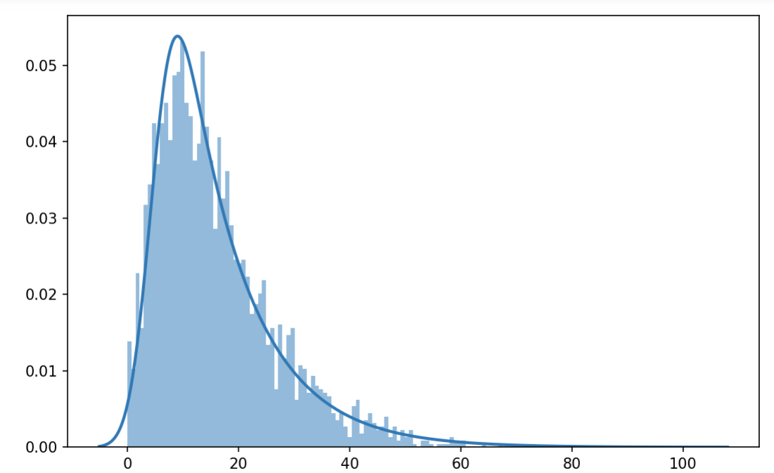
The exponential normal distribution has three parameters which control the shape of the distribution. Each year, the parameters are fit to the end of season EPA ratings using maximum likelihood estimation. The percentiles of the distribution are then used to map the team's EPA rating to year normalized EPA rating, defined by another exponential normal distribution fit to EPA ratings from all years. A separate exponential distribution is used to better approximate the percentile of the top 5% of teams.

Given the methodology, the year normalized EPA is only available at the end of the season.

To date, the most dominant single season in FRC history is 1114 is 2008 (and it's not particularly close). More detailed write-up on year-normalized EPA coming soon!

Results

Detailed results and discussion are available on a separate post here. The main prediction accuracy results are summarized in the table below. EPA significantly outperforms the Elo and OPR models.

Comparison of Historical Prediction Performance (2002 - Present)

Year		Wins Baseline	OPR	Caleb Sykes Elo	EPA
Year	N	Acc	Acc	Acc	Acc
2016	13320	65.23%	68.90%	70.05%	71.87%
2017	15442	61.66%	64.73%	64.83%	65.63%
2018	16930	68.29%	70.78%	73.93%	73.61%
2019	18035	65.68%	69.66%	70.09%	71.78%
2020	4571	61.96%	70.42%	69.62%	72.03%
2022	14629	69.18%	76.70%	75.71%	77.47%
2016 - 2022		65.80%	70.13%	70.85%	72.04%

Include metrics:

Accuracy

Brier Score

Show:

Only Champs

Entire Season

Start Year:

2016

End Year:

2022

Google Sheets Link: here

Reproducibility

Statbotics is open-source, and the code responsible for calculating EPA ratings is available here. I am working on a standalone Jupyter Notebook that will allow for easier experimentation and reproduction. Please reach out or create/upvote a Canny issue to prioritize.