Strength of Schedule

How can we use EPA to measure strength of schedule? We propose three metrics and briefly explore some results.

What is Strength of Schedule?

Strength of Schedule (SOS), measures how difficult a team's schedule was or will be. An easy schedule means that the team played with on average strong alliance partners, and against on average weak opponents. Conversely, a difficult schedule means that the team played against tougher opponents. Notably, SOS is not a measure of a team's intrinsic strength, but rather the external factors that contribute to a team's final ranking. In this post, we will explore three different ways to measure SOS, and explore some interesting results from 2022 champs.

Strength of Schedule Metrics

Qualities of a Good SOS Metric

When designing a strength of schedule metric, I prioritized certain attributes. This is neither a comprehensive nor objective list, but rather a list of attributes that I thought were important.

Explainable: The metric should be easy to understand and have some real-world interpretation. This allows for easy communication of the metric's meaning.
Fair: The metric should be indifferent to a team's EPA rating, allowing for easy comparison between teams. A strong team does not have an "easy" schedule just because they are projected to win more matches.
Percentile Based: Each metric should be a percentile, denoting what percentage of random schedules are easier than the team's actual schedule. This also allows multiple metrics to be averaged together to create a composite SOS metric.

Caleb Sykes also has a great post on strength of schedule metrics.

Methodology

Each metric follows the same general framework. First, we generate N random schedules to represent the possible schedules that could have been played. I use Chezy Arena to generate well balanced schedules and randomly assign teams to slots. We then calculate some quantity of interest for each team for each schedule. We do the same for the actual schedule. We can then compare the quantity of interest from the actual schedule with its distribution over the random schedules to get a percentile. This is the SOS metric.

Each metric takes as input a mapping between teams and their perceived strength to compute the quantity of interest. Specifically, we explore using a team's EPA rating from both before the event and after the event. The SOS metrics from before the event measures the expected difficulty of the schedule upon release, whereas the SOS metrics from after the event measures the actual schedule difficulty based on how teams indivdiually performed.

Metric 1: Δ RP

This method is the simplest. Using the event simulator, simulate each match and compute the number of ranking points each team is expected to earn. The metric is the difference between the simulated RPs of the actual schedule and the average of random schedule simulations. The RP Percentile denotes the percentage of random schedules with a lower expected ranking point total than the actual schedule.

Metric 2: Δ Rank

In a similar vein, we can compute the difference in rank between the actual schedule and the average of random schedule simulations. This is slightly different than the previous metric because rank may be nonlinearly related to ranking points. The Rank Percentile denotes the percentage of random schedules with a lower expected rank than the actual schedule.

Metric 3: Δ EPA

This method is slightly different than the previous two. In a perfectly balanced schedule, your alliance partners should be approximately as good as your opponents. We can measure deviations from this ideal by computing the average EPA of your alliance partners and opponents. Since a team has two alliance partners and three opponents, temporarily assume the team has an average EPA and compute the difference in alliance EPAs.

$\text{Δ EPA}=\text{Avg EPA} + 2 \times (\text{Avg Alliance EPA}) - 3 \times (\text{Avg Opponent EPA})$

Δ EPA can be interpreted as the headwind or tailwind a team experiences as a result of their schedule. For example, a team with a Δ EPA of 10 is expected to outscore opponents by 10 points just by being average. To compute the percentile, we approximate the distribution of EPAs at the event as a normal distribution. If

$\text{EPA}\sim\mathcal{N}(\mu,\sigma^2)$

, then

$\text{Δ EPA}\sim\mathcal{N}(0, 5\times\sigma^2)$

(since one EPA is fixed). Measuring

$\sigma$

from the event data and dividing by

$\sqrt{n}$

(where n is the number of matches per team), we can approximate the distribution of Δ EPA. We can then compute the percentile of the actual schedule using the cumulative distribution function.

Composite Metric

All three metrics, along with some intermediate calculations, are available on the Strength of Schedule tab of events with a released match schedule. We can also compute a composite SOS metric by averaging the three metrics together. This metric has the least noise while still being explainable and fair. While the composite SOS metric is the primary metric recommended, understanding each component can help explain the final results.

Sample Results

In this section I will explore some interesting results from the 2022 champs divisions.

Carver Division

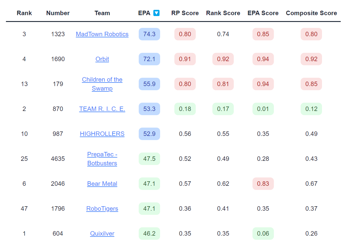
Coming into the event, 1323 and 1690 were two of the top teams in the world and had a significantly higher EPA than the rest of the field. However, once the schedule released, 1323, 1690, and 179 were given challenging schedules, as reflected in their high composite SOS. Meanwhile, 604 and 870 had strong robots and relatively easier schedules, eventually seeding first and second and breaking up the possible 1323/1690 alliance. Looking more closely, 870's EPA percentile was 0.01, indicating only 1% of random schedules had a more favorable difference between alliance and opponent EPAs. This was one of the more unbalanced schedules in recent years. Still, 870 was 4th in EPA and 604 was 9th in EPA entering the event, while teams with even more favorable schedules did not crack the top 10.

Hopper Division

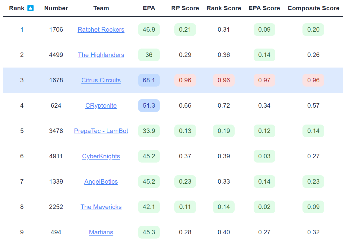
Despite a very challenging schedule by all three metrics, 1678 was able to rank 3rd in Hopper, eventually making it to Einsteins and continuing their legendary streak. Most of the other teams in the top 10 had relatively easy schedules, with an average composite SOS of 0.26. I include this example to show that a challenging schedule does not necessarily doom a team, especially if they have a very strong robot.

Turing Division

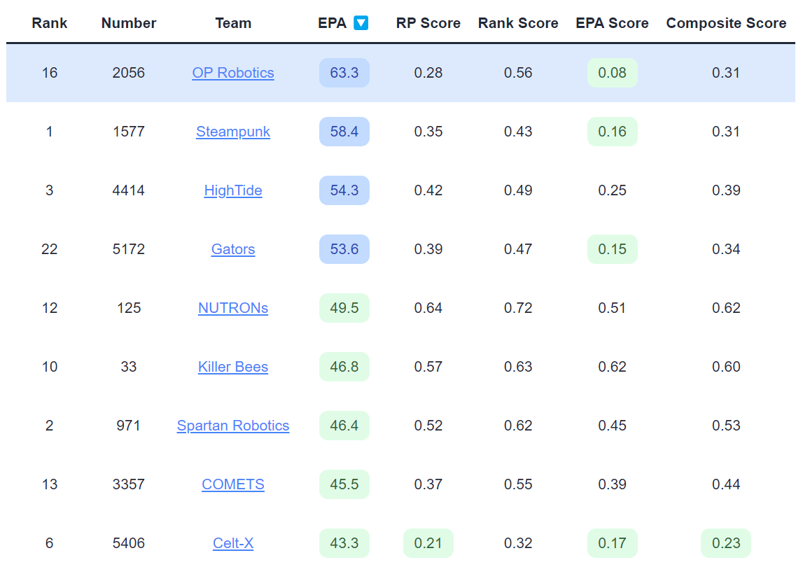
Looking at 2056's SOS of 0.31, their schedule seems slightly easier than average. But when we look at the individual metrics, we see that their Δ EPA was 0.08 (great!) while their Δ Rank was only 0.56 (pretty average). Somehow, their average alliance partners were better than their average opponents, but they were expected to seed slightly lower than their average random schedule. This is a very interesting result, and partly explained by Qual Match 28. In this match, the EPA model predicts a landslide victory for 2056, and indeed they win by 133 points. While this greatly benefits their Δ EPA, a win is always worth 2 ranking points, and their remaining matches are all a lot closer. This exercise highlights the importance of understanding the individual metrics and how they interact.

Conclusion

In this article, I introduced three metrics for measuring the strength of schedule and a composite metric that combines them. I also explored some interesting results from the 2022 champs divisions. I hope that the strength of schedule feature and this article will help teams understand their schedules and make better decisions about their strategy. As always, if you have any questions or comments, feel free to reach out to me!